| Release 1.1 | 20 August 2008 | Associated with Catalogue version 1.0 (released 22 August 2007) |
Prepared by the XMM-Newton Survey Science Centre Consortium.) |
||
This User Guide refers directly to the full FITS and plain-text formats of the catalogue. It provides a detailed account of the production and contents of the catalogue. Users interested in the main properties of the catalogue will find the summary and sections 1 & 5 of most immediate interest.
2XMM is a catalogue of serendipitous X-ray sources from the European Space Agency's (ESA) XMM-Newton observatory, and has been created by the XMM-Newton Survey Science Centre (SSC) on behalf of ESA. The pre-release catalogue, 2XMMp, made public in July 2006, was essentially a subset of this full 2XMM catalogue.
The catalogue contains source detections drawn from 3491 XMM-Newton EPIC observations made between 2000 February 3 and 2007 March 31; all datasets included were publicly available by 2007 May 01 but note not all public observations are included in this catalogue. The total area of the catalogue fields is ~ 560 deg2, but taking account of the substantial overlaps between observations, the net sky area covered independently is ~ 360 deg2.
The processing used to generate the catalogue is based on the pipeline developed for the re-processing of all XMM observations. The new pipeline includes a number of significant improvements over the previous data processing system (as used by the SSC in routine processing of XMM-Newton data on behalf of ESA). These improvements include a more sensitive source detection scheme using exposures of all cameras, the detection and parameterization of extended sources and the extraction of spectra and time series for the brightest sources.
The 2XMM catalogue contains 246897 X-ray source detections above the processing likelihood threshold of 6. The 246897 X-ray source detections relate to 191870 unique X-ray sources, that is, a significant fraction of sources (27522) have more than one detection in the catalogue.
As part of extensive quality evaluation for the catalogue, each field has been visually screened. Regions where there were obvious deficiencies in the automatic processing were identified, and all sources within those regions were flagged. There are 199359 out of 246897 detections which have not received such a flag (and can thus be considered to be 'clean').
The present catalogue also distinguishes between extended emission and point-like detections. Parameters of detections of extended sources are only reliable up to the maximum extent measure of 80 arcseconds. There are 20837 detections of extended emission, of which 3836 are 'clean' (i.e., have not received a manual flag).
For 38320 detections spectra and time series were automatically extracted during processing, and a χ2-variability test was applied. 2307 detections in the catalogue are considered variable at a probability of 10-5 or less based on the null-hypothesis that the source is constant.
The median flux (in the total photon-energy band 0.2 - 12 keV) of the catalogue detections is ~ 2.5 × 10⁻¹⁴ erg/cm2/s; in the soft energy band (0.2 - 2 keV) the median flux is ~ 5.8 × 10⁻¹⁵, and in the hard band (2 - 12 keV) it is ~ 1.4 × 10⁻¹⁴. About 20% have fluxes below 1 × 10-14 erg/cm2/s. The positional accuracy of the catalogue detections is generally < 5 arcseconds (99% confidence radius). The flux values from the three EPIC cameras are overall in agreement to ~ 10% for most energy bands.
Pointed observations with the XMM-Newton Observatory detect significant numbers of previously unknown 'serendipitous' X-ray sources in addition to the proposed target. Combining the data from many observations thus yields a serendipitous source catalogue which, by virtue of the large field of view of XMM-Newton and its high sensitivity, represents a significant resource. The serendipitous source catalogue enhances our knowledge of the X-ray sky and has the potential for advancing our understanding of the nature of various Galactic and extragalactic source populations.
The 2XMM catalogue is ~ 6 times larger than the 1XMM catalogue released in 2003 and over 50% larger than the pre-release version, 2XMMp. (The difference between 2XMM and 2XMMp arises from both a longer observation baseline (~ 1 year) and the more inclusive screening regime for 2XMM which was more cautious for 2XMMp. )
The 2XMM catalogue is the largest X-ray source catalogue ever produced, containing almost twice as many discrete sources as either the ROSAT survey or pointed catalogues. 2XMM complements deeper Chandra and XMM-Newton small area surveys, probing a large sky area at the flux limit where the bulk of the objects that contribute to the X-ray background lie. The 2XMM catalogue provides a rich resource for generating large, well-defined samples for specific studies, utilizing the fact that X-ray selection is a highly efficient (arguably the most efficient) way of selecting certain types of object, notably active galaxies (AGN), clusters of galaxies, interacting compact binaries and active stellar coronae. The large sky area covered by the serendipitous survey, or equivalently the large size of the catalogue, also means that 2XMM is a superb resource for exploring the variety of the X-ray source population and identifying rare source types.
The production of this catalogue has been undertaken by the XMM-Newton Survey Science Centre (SSC) consortium in fulfillment of one of its major responsibilities within the XMM-Newton project. The catalogue production process has been designed to exploit fully the capabilities of the XMM-Newton EPIC cameras and to ensure the integrity and quality of the resultant catalogue through rigorous screening of the data.
The selection of XMM-Newton observations for processing in the 2XMM catalogue pipeline is based on the desire to re-process all available observations with the latest available data processing system and calibration data. All observations that have a public release date prior to 2007 May 01 are eligible for inclusion. Table 2.1 gives the list of the final 3491 observations which are included in the catalogue, while Table 2.2 gives a list of observations which were public by 2007 May 01 and have EPIC images suitable for source detection but which could not be included in the catalogue. A short comment on the reason for exclusion is given as well.
It should be noted that the field of view (FOV) of an XMM observation (the combined three cameras) has a radius ~ 17 arcminutes, and that contiguous multi-FOV spatial coverage is rare.
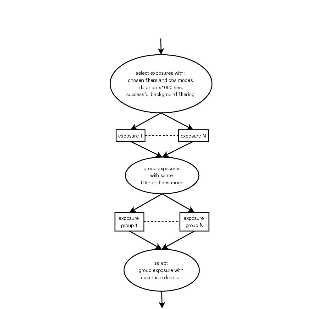
Most XMM-Newton observations comprise a single exposure by each of the three EPIC cameras (a significant number of observations have multiple exposures and/or do not include exposures with one or more of the three cameras). For each observation, exposures were selected for each of the three EPIC cameras for processing using the following criteria:
| (i) | An exposure must have > 1000 seconds duration. |
| (ii) | The exposure must have been taken through a scientifically useful filter. In practice this rejected all exposures for which the filter position was closed, calibration or undefined. The possible filters used in the observations selected for the catalogue are Medium, Thick, Thin1, Thin2 (PN only), and Open. For a detailed description of the filters see 3.3.6 EPIC filters and effective area in the XMM user hand book. |
| (iii) | The exposure must have been taken in a mode which could usefully be processed by the detection stage. PN small window modes were rejected since the effective FOV in these modes is small, making the background fitting stage of the source detection problematic. For the MOS nearly all modes, including those modes in which the area of the central CCD was windowed or missing (e.g., timing modes, here 'Fast Uncompressed') or modified ('Refreshed Frame Store' mode), were included. The observing modes used in the observations selected for the catalogue are given in Table 2.3. For a detailed description of the modes see 3.3.2 Science modes of the EPIC cameras in the XMM user hand book. |
| (iv) | Background filtering (see Sec. 3.1.1 c)) must have been successfully applied. Cases, where the sum of all Good Time Intervals (hereafter GTIs) was less than 1000s, were rejected as unusable. Without background filtering the source detection is typically of limited value due to the much higher net background. |
| (v) | After background filtering has been applied, each of the five images of an exposure (energy bands 1 - 5) must have at least one pixel per image with more than one event. |
Where more than one exposure with a particular camera met the above selection conditions, all exposures with the same filter and data mode were merged and then the exposure group with maximum good exposure time was chosen for the source detection. The zoom-in flow chart below visualizes the selection procedure.
 |
The processing of the observations was facilitated through an improved pipeline configuration over the one previously used for the routine production processing of observations. This new processing pipeline was used to re-process all available observations up-to-date and has become the new routine pipeline after the re-processing was concluded.
After creation of the pipeline data products (Sec. 3.1), the catalogue file was constructed to contain key columns from the source lists plus additional columns which include observation-level meta-data for each source as well as further processing and analyses (Sec. 3.2). Additional products for each source were created to facilitate data access (Sec. 3.3).
Throughout the documentation references to catalogue columns are marked as links to their description. The prefix 'ca_' in a column name indicates a wildcard for any of the three EPIC cameras, i.e., 'ca' is to be replaced by 'PN,' 'M1' or 'M2'; it can also stand for 'EP' (that is, EPIC) where applicable. Some of the column names also include an energy band identifier ('_b_', where b = 1,2,3,4,5,6,7,8,9) which is typically not explicitly indicated. The four hardness ratios are identified by the designator 'n' (n = 1,2,3,4).
The zoom-in flow chart below gives an overview of the processing steps from the XMM-Newton observation to the final observation source list as described in this section. The 'exposure group selection' is described in Sec. 2.2.
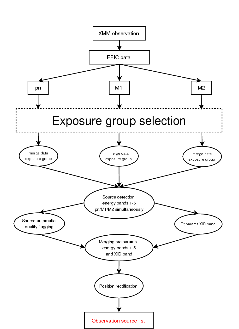 |
The following sections describe the individual steps taken within the pipeline processing chain leading to images on which source detection could be performed (Sec. 3.1.1), the source detection procedure (Sec. 3.1.2), the rectification of the positions (Sec. 3.1.3), and the extraction of source-specific products (Sec. 3.1.4). Note that these sections are applicable to all observations processed with this pipeline, indpendent on whether they have been used in the catalogue or not.
1. A first pass constructs a high energy background lightcurve selecting events with the (XMMEA_22 = REJECT_BY_GATTI & XMMEA_EM = GOOD_MOS_EVENTS) flags set.
2. GTIs are made by filtering the high energy background lightcurve using the MOS flare threshold (2 counts/arcmin2/kilosecond). These GTIs are used to define the time regions in which bad pixel searching occurs.
3. All GTIs with a duration of less than 100 seconds are excluded.
4. The SAS task embadpixfind is used to locate dark pixels in each MOS CCD (using events which have not been filtered through the flare GTIs).
5. If no flare GTIs were made the SAS task embadpixfind is used to locate bright pixels.
6. If flare GTIs do exist the events are filtered through the flare GTIs and then embadpixfind is used to locate bright pixels.
7. The SAS task badpix is run on each CCD event file in order to add a bad pixel extension.
8. The intervals in the global GTI file are aligned with the event list and merged with the CCD GTIs.
9. Attitude correction is applied to the individual events to convert raw CCD pixel coordinates, through camera coordinates, to celestial coordinates.
10. Raw event pulse height values are converted to rectified event energies.
11. Unwanted events are filtered out before lists are merged.
12. The per-CCD event lists are merged into one per camera.
13. Filter the good imaging events into final event lists.
14. Copy the Calibration Index File (CIF) into a separate extension in the event list.
15. Make a second pass high energy background lightcurve selecting events as before, but now with the bad pixels excluded.
16. Create flare GTIs using the MOS flare threshold.
17. Filter the event files through GTIs into final event files.
1. The SAS task badpixfind is run to create a mask of non-source pixels to be used in generating a high energy background lightcurve.
2. badpixfind is run on each CCD to locate bright and dead pixels.
3. Attitude correction is applied to the individual events to convert raw CCD pixel coordinates, through camera coordinates, to celestial coordinates.
4. Raw event pulse height values are converted to rectified event energies.
5. Filter events by selecting events with the (XMMEA_EP = PN_GOOD_EVENTS) flags set.
6. Filter the CCD event files on the HK GTIs and merge into one.
7. Copy the CIF into a separate extension in the event list.
8. Make a high energy background lightcurve using events with energies between 7 keV & 15 keV events and excluding bad pixels by using the previously created pixel mask.
9. Create flare GTIs using the PN flare threshold (10 counts/arcmin2/kilosecond) for use in later processing stages.
The MOS high energy background lightcurves were produced from GATTI-flagged (essentially events with energies above 14 keV), single-pixel events from the outer CCDs. After binning the lightcurve, the GTIs were selected by imposing a rate threshold of 2 counts/arcmin2/ksec.
The PN high energy background lightcurves were produced in the 7.0 - 15 keV energy range. After binning the lightcurve, the GTIs were selected by imposing a rate threshold of 10 counts/arcmin2/ksec.
1. Exclude from the flare GTIs all intervals with duration less than 100 seconds.
2. For each energy band make a counts image. The images are 600 × 600 pixels with 4-arcsecond pixel sides. The images are tangent plane projections of celestial coordinates. Note that the energy bands have changed slightly with respect to previous processing: the old band 2 is split into two bands now (0.5 keV - 1.0 keV and 1.0 keV - 2.0 keV), while the old bands 4 and 5 have been merged into a single band. The definitions of all the new energy bands are given in Table 3.1 below.
| Basic energy bands: | 1 | = | 0.2 - 0.5 keV | ||
| 2 | = | 0.5 - 1.0 keV | (formerly part of band 2) | ||
| 3 | = | 1.0 - 2.0 keV | (formerly part of band 2) | ||
| 4 | = | 2.0 - 4.5 keV | (formerly band 3) | ||
| 5 | = | 4.5 - 12.0 keV | (formerly bands 4 and 5) | ||
| Broad energy bands: | 6 | = | 0.2 - 2.0 keV | soft band, no images made | |
| 7 | = | 2.0 - 12.0 keV | hard band, no images made | ||
| 8 | = | 0.2 - 12.0 keV | total band | ||
| 9 | = | 0.5 - 4.5 keV | XID band | ||
3. Event selection for PN images is PATTERN <= 4 and RAWY > 12 with events ON_OFFSET_COLUMN excluded. Band 1 images have the additional stricter requirement PATTERN = 0, while band 8 images have PATTERN = 0 below 0.5 keV. Band 1 - 5 images have also events OUT_OF_FOV excluded.
4. For MOS band 1 - 5 and 8 images no PATTERN selection is made beyond the 0 - 25 selection made in the event lists. Events OUT_OF_FOV are excluded for band 1 - 5 images.
5. Make exposure images corresponding to bands 1 - 5 count images
Source detection is performed simultaneously on images in the energy bands 1 - 5 and from the three EPIC cameras. For observations having multiple exposures from the same camera, exposures are merged by filter and observing mode, and for each camera the merged ('added') exposure with the longest integration time is used for source detection (cf. Sec. 2.2).
In the fitting routine source parameters are determined individually for the three cameras [PN,M1,M2] in the energy bands 1 - 5 as well as the XID band (cf. Table 3.1). These parameters are then combined to obtain camera dependent parameters in band 8 as well as all-EPIC parameters. On the other hand, the fitted source position is constrained to be the same in all bands and cameras.
Exposure maps hold the effective exposure time for each detector point
(see Sec. 3.1.1). They are created by the
SAS task eexpmap
for each EPIC camera and energy bands 1 - 5 using the latest
calibration information on the mirror vignetting, quantum efficiency and
filter transmission. The exposure maps (see ca_EXP) are corrected for bad
pixels, bad columns and CCD gaps as well as being multiplied by an
out-of-time factor (oot_factor):
| oot_factor = | 0.9411 | for PN PrimeFullFrame modes, |
| 0.97815 | for PN ExtendedFullFrame modes, | |
| 1.0 | for all other PN and M1/M2 modes. |
See SSC-LUX-SP-0004.pdf, Sec. 6.5.2.6, for more details.
The SAS task emask is used to create a detection mask for each camera. Detection masks define the area of the detectors which is suitable for source detection. Only the areas of the detector where the exposure is at least 50% of the maximum exposure have been used for source detection (based on unvignetted exposure maps).
The SAS task eboxdetect is used to create a preliminary source list. It has two operation modes: local and map detection. At this stage eboxdetect is run in local mode and performs a sliding box cell detection (box size 5 × 5 pixels) on the detector areas defined by the detection masks. Eboxdetect in local mode uses a local background that is determined in a frame around the search box. All sources with a 0.2 - 12 keV EPIC detection likelihood above 5 are included in the output source list.
The SAS task esplinemap
is used to create background maps for each camera and energy bands
1 - 5. Using a cut-out radius dependent on source brightness,
esplinemap blanks out the areas of the images where sources were
detected by eboxdetect in local mode. Then esplinemap
performs 12 × 12 nodes spline fits on the resulting
source-free images to calculate a smoothed background map for the entire
images (ca_BG).
A second pass of eboxdetect is carried out in map mode. It creates a new source list using this time the background maps generated by esplinemap, increasing thereby the source detection sensitivity as compared to the local detection step. The box size is again set to 5 × 5 pixels. All sources with a 0.2 - 12 keV EPIC detection likelihood above 5 are included in the eboxdetect map mode source list.
The sources detected by eboxdetect in map mode are passed on to
the SAS task emldetect. Emldetect
does not perform source detection, instead it calculates PN/M1/M2 source
parameters in the bands 1 - 5 by fitting the instrumental point
spread function (PSF) convolved with a source extent model to the
distribution of counts of the sources detected by eboxdetect (in
map mode) simultaneously in the bands 1 - 5 and the three
cameras. The extent model used is a beta-model profile, see SSC-AIP-TN-003.pdf for more details on the
extended source detection. Free parameters of the fits are source
positions, extent (ep_EXTENT), and count rates
(ca_RATE). Positions
and extent are constrained to be the same in all energy bands and for all
cameras while count rates are obtained from the best fit value for each
camera and energy band. Detection likelihoods (ca_DET_ML) and extent
likelihoods (ca_EXTENT_ML) are derived as
well.
In a second loop, emldetect attempts to fit two PSFs to sources detected as extended, and for those detections where the split improved the likelihood of the fit the (point) source parameters were re-calculated.
Emldetect uses the multiband exposure maps (Sec. 3.1.2 a)) to correct the count rates for vignetting and losses due to inter-chip gaps and bad pixels/columns as well as for losses in the PN due to events arriving during readout times (out of time events):
count_rate = source_counts / exp_map .
Emldetect derives four camera-specific X-ray colours known as hardness ratios (HR), which are obtained for each camera by combining corrected count rates from different energy bands. Each hardness ratio, HRn, is obtained as
HRn = (RATE_b - RATE_a) / (RATE_b + RATE_a),
where RATE_a and RATE_b are the corrected count rates in
energy bands a and b (see ca_b_RATE). Energy
bands 1 & 2 are used to obtain ca_HR1, 2 & 3 for ca_HR2, 3 & 4 for ca_HR3, and 4 & 5 for
ca_HR4.
Count rates and therefore hardness ratios are camera dependent. In addition they depend on the blocking filter used for the observation, especially the HR1. This needs to be taken into account when comparing hardness ratios for different sources. Note that a large fraction of the hardness ratios are calculated from marginal or non-detections in at least one of the energy bands. Consequently, individual hardness ratios should only be deemed reliable if the source was above the detection likelihood threshold in both energy bands, else they have to be treated as upper limits.
Emldetect calculates observed source fluxes (ca_FLUX) in bands 1 - 5
in units of [erg/s/cm2], using the count rates (ca_RATE) in those bands using the
following expression:
Flux = Rate / ECF ,
where the ECF is an energy conversion factor (to 'convert' count rates to fluxes). ECFs have been calculated using the most recent calibration matrices for MOS, and v6.7 response matrices (RMFs) for the PN. They have been calculated assuming a spectral model of an absorbed power-law with absorbing column density Nh = 3.0 × 1020 cm2 and continuum spectral slope Gamma = 1.7 (see CAL-TN-0023-v2.0.pdf).
ECFs for each camera, energy band, and filter in units of [1011 cts cm2/erg] are given in Table 3.2. EPIC-PN Thin1 and Thin2 filters have the same transmission.
| Camera | Band | Open | Thin | Medium | Thick |
| PN | 1 | 16.1784 | 8.95403 | 7.82028 | 4.71096 |
| 2 | 10.0418 | 8.09027 | 7.83782 | 6.02015 | |
| 3 | 6.17030 | 5.88255 | 5.78272 | 5.00419 | |
| 4 | 1.95859 | 1.92805 | 1.90529 | 1.80647 | |
| 5 | 0.555924 | 0.555226 | 0.554529 | 0.547205 | |
| 9 | 5.07412 | 4.53836 | 4.43953 | 3.74772 | |
| MOS-1 | 1 | 3.15223 | 1.80399 | 1.60150 | 1.06500 |
| 2 | 2.27921 | 1.88017 | 1.82853 | 1.48465 | |
| 3 | 2.14933 | 2.05034 | 2.01594 | 1.79446 | |
| 4 | 0.757786 | 0.746128 | 0.737800 | 0.707822 | |
| 5 | 0.143619 | 0.143340 | 0.143131 | 0.141213 | |
| 9 | 1.54600 | 1.42040 | 1.39361 | 1.23264 | |
| MOS-2 | 1 | 3.17622 | 1.81179 | 1.60670 | 1.06620 |
| 2 | 2.28390 | 1.88369 | 1.83088 | 1.48818 | |
| 3 | 2.15017 | 2.05117 | 2.01594 | 1.79530 | |
| 4 | 0.761672 | 0.750569 | 0.741687 | 0.711708 | |
| 5 | 0.151083 | 0.150769 | 0.150560 | 0.148537 | |
| 9 | 1.54912 | 1.42326 | 1.39647 | 1.23524 |
Note that all count rates (ca_RATE) and fluxes (ca_FLUX) correspond to the flux
in the entire PSF and do not need any further corrections for PSF
losses.
Band 8 source parameters are derived from the
combination of parameters from bands 1 - 5. For
details on how each parameter was obtained see the column descriptions
for the source
parameters.
Detection likelihood values (ca_DET_ML) as calculated by
emldetect are based on the likelihood ratio described by Cash (1979) and are defined as
DET_ML = - ln(P), where P is the probability of the
detection occurring by chance. To allow comparisons of source detection
runs with different source parameters, the detection likelihoods in
emldetect are given in the form of 'equivalent' detection
likelihoods, i.e., they are corrected for the number of free fit
parameters. All sources (as detected by eboxdetect map mode) with
0.2 - 12 keV EPIC detection likelihoods greater than 6
as determined by emldetect are included in the output source
list.
Band 9 source parameters are for the XID band (0.5 - 4.5 keV). Instead of combining parameters from bands 2, 3 and 4, which will produce overall larger source parameter errors, the SAS task emldetect is run a second time using merged images, exposure maps and background maps from bands 2 - 4. Source positions are kept fixed at the values determined previously, and a likelihood threshold of zero is used to ensure that band 9 parameters are obtained for all sources detected in the first run of emldetect. The output source list contains only band 9 parameters with errors determined directly from the merged images.
One of the improvements over the previous processing pipelines is the
setting of automatic flags by the SAS task dpssflag;
based on the available information in the emldetect source list it
writes a string of twelve different flags back into the source list
(ca_FLAG) to indicate
various conditions (note that only nine of these are used in the pipeline
processing). Because the decision tree had to be simple these flags should
be understood mainly as a warning. In particular, sources with a low
coverage on the detector, sources in problematic areas (near a bright
source or within an extended source) as well as sources near artefacts like
the known bright MOS-1 corner or the occasionally bright low gain columns
of the PN are flagged. In addition, an attempt was made to identify
spurious extended sources which can often be found near bright sources,
within complicated extended emission, or generally in areas where the
background changes considerably on a small spatial scale and the spline
maps can not adapt well enough. The nine flag positions have been assigned
the meanings given in Table 3.3a (note that
flags 1, 8, and 9 are camera dependent):
| 1 | Low detector coverage | ca_MASKFRAC < 0.5 |
| 2 | Near other source | R ≤ 65 * SQRT (EP_RATE); R(min) = 10", R(max) =
400" |
| 3 | Within extended emission | R ≤ 3 * EP_EXTENT; R(max) = 200" |
| 4 | Possible spurious extended source near bright source | Flag 2 is set and EP_CTS(min) = 1000 for the causing
source |
| 5 | Possible spurious extended source within extended emission | R ≤ 160" and fraction of rate wrt causing source is 0.4 |
| 6 | Possible spurious extended source due to unusal large single-band DET_ML | Fraction of ca_b_DET_ML wrt the sum of all
≥ 0.9 |
| 7 | Possible spurious extended source | At least one of the flags 4, 5, 6 is set |
| 8 | On bright MOS-1 corner or bright low gain PN column | |
| 9 | Near bright MOS-1 corner | R ≤ CUTRAD = 60" of a bright pixel the corner |
The default value of every flag is F for False. When a flag was set it means it has been changed to T for True.
The task dpssflag sets all flags except the camera-specific flags (i.e., flags 2,3,4,5,6,7) on the summary row (EPIC band 8) which are then propagated backwards to the individual cameras and bands.
The emldetect source list for the bands 1 - 5 is
merged with the emldetect XID source list into a common list by
the SAS task srcmatch.
The output table consists of a single row per detection with parameters
from both input lists in different columns. The task srcmatch also
calculates band 1 - 5 EPIC fluxes (EP_FLUX), EPIC hardness ratios
(EP_HRn), and their
respective errors.
The task srcmatch introduces flag columns which are later
populated by the pipeline, e.g., for sources where source-specific products
(Sec. 3.1.4) have been made (TSERIES and SPECTRA).
The SAS task eposcorr correlates the X-ray positions from an observation (as determined by the fitting routine of emldetect) with catalogued optical positions and minimizes the positional offsets by applying a translation and rotation to the X-ray positions. For the catalogue pipeline the srcmatch source lists were correlated with the USNO B1.0 optical catalogue. The correlation allows offsets in RA/DEC of up to 10 arcseconds while all optical sources more than 15 arcseconds from an X-ray source are removed prior to correlation.
The SAS task evalcorr evaluates the quality of the position rectification of eposcorr. For 2XMM the following empirically determined condition was used to accept the refined astrometric solution:
POSCOROK is set to True by evalcorr if
LIK_HOOD > 9.0 + ( 2.0 * LIK_NULL ) ,
where LIK_HOOD and LIK_NULL are determined by the SAS task eposcorr. LIK_NULL is the likelihood calculated for purely coincidental X-ray/optical matches in a given observation, i.e., if there were no true counterparts.
If POSCOROK is set to True the columns RA and DEC give the corrected X-ray positions
calculated by eposcorr. If the refined astrometric solution was
not accepted the columns RA and DEC are the same as the
uncorrected values RA_UNC and DEC_UNC (as determined by
emldetect). POSCOROK also determines the value to the parameter
SYSERRCC which is the nominal value of the systematic 1-sigma
position error for XMM-Newton fields.
In the pipeline products as well as in 2XMMp, the value of SYSERRCC was estimated from the width of the distributions of position shifts found in eposcorr runs. It is 0.5 arcseconds for all detections in a field for which an acceptable astrometric correction using eposcorr was determined (that is, POSCOROK is True). For fields for which no acceptable astrometric correction using eposcorr was determined (that is, False), the value of SYSERRCC is 1.5 arcseconds.
For the 2XMM catalogue, a re-analysis of the astrometric
properties has led to a new determination of the systematic 1-sigma position error,
reflected in the new (catalogue-only) parameter SYSERR, see Sec. 3.2.2 for details.
The new pipeline automatically extracts time series and spectra for the
brighter detections (EPIC counts ≥ 500. Where the detection was
only observed with one or two cameras the equivalent EPIC counts were
calculated using the PN to MOS count ratio 3.5 : 1). All
exposures that passed the filtering (i) - (v) in Sec. 2.2 were used for
extraction. Source-specific products were made when the following
camera-specific conditions were met: (i) ca_MASKFRAC ≥ 0.5,
and (ii) ca_DET_ML
≥ 15. Detection flags (see Sec. 3.1.2 h)) were not taken into
account.
The source counts were extracted from a circular aperture with radius 28", and the background counts were extracted from an annulus around the detection position with r (min) = 60" and r (max) = 180". PATTERN selection is the same as for image creation (PN: PATTERN <= 4, MOS: PATTERN <= 12). Event FLAG selection was done according to the recommendations: FLAG = 0 for the PN, XMMEA_EM for MOS time series, and XMMEA_SM for MOS spectra. The energy range for the extraction of all products is 0.2 - 12.0 keV.
While time series are filtered only by instrumental GTIs (see Sec. 3.1.1 a) and b)), spectra are also filtered for the flare background (see Sec. 3.1.1 c)). The variability tests, however, exclude times where the flare background is high.
The bin size for the time series was chosen in such a way that the PN bins contain at least 18 counts and the MOS bins at least 5 counts as derived from the source lists. Note that these are background subtracted according to the background maps determined in the source detection process, see Sec. 3.1.2 d). The minimum bin size is 10 seconds, and all other bin sizes are rounded up to an integral multiple of 10.
To test for variability a χ2-test (suitable
for binned data) was used with the Pearson's approximation for Poissonian
data. Times with high background flaring were excluded from the test. The
SAS task ekstest
writes four keywords into the header of the time series file, namely
CHI2PROB for the
probability, CHISQUAR for the χ2-statistic, N_POINTS for the
number of bins used in the test, and AVRATE for the mean rate in the number
of bins used for the test.
The spectral products for each selected detection in 2XMM are (i) a grouped source spectrum (20 counts/bin where energies below 0.35 keV as well as energies in the PN around the copper line at 8.05 keV are set to 'bad'), (ii) a background spectrum, (iii) a source ARF (auxillary response file), and (iv) a spectral plot made using XSPEC. A keyword in the header of the source spectrum file indicates the name of the canned RMF (response matrix file) that can be used with this detection.
The time series products for each selected detection in 2XMM are (i) a time series file containing the source minus background and background arrays (corrected for exposure, cosmic rays, and dead time) as well as the keywords regarding the variability, and (ii) a plot of the time series and the background made by the SAS task elcplot.
The available products are identified by their observation ID (OBS_ID), exposure ID and the
observation-specific source number SRC_NUM in the hexadecimal
system. Further details and a discussion of the limitations of an automatic
extraction can be found in SSC-LUX-RE-0155.pdf.
Most of the catalogue columns are derived from information in the lists output by the srcmatch task (see Sec. 3.1.2 i)); some further information has been extracted from the emldetect source lists (see Sec. 3.1.2 f)). Additional columns, derived from other products and obtained by further processing, are explained in this section.
The catalogue includes meta data derived from keywords in the source
list files to help characterize the detections. These are the observation
ID (OBS_ID); revolution
number (REVOLUT); the
beginning and end of the observation in Modified Julian Date format
(MJD_START and MJD_STOP); filter (ca_FILTER) and submode (ca_SUBMODE); note that the
latter two apply to all exposures in a merged set, see Sec. 2.2 .
A detailed analysis of the 2XMM catalogue has been used to refine the
value of the systematic 1-sigma error for XMM-Newton sources. This is
reflected in the SYSERR
parameter which replaces the nominal SYSERRCC value used in 2XMMp (see Sec. 3.1.3 ). The analysis is based on a
comparison between the 2XMM X-ray and SDSS optical positions for a sample
of ~ 1000 broad emission line quasars (the Sloan
DR5 Quasar Catalog) which is expected to have neglible contamination by
chance positional matches (the SDSS positions are known to better than 100
milliarcseconds). This analysis demonstrates that the statistical
properties of this sample, which is believed to be representative of the
whole catalogue, can be well described with an additional systematic
positional error component with a fixed value SYSERR = 0.35 arcseconds for
all fields for which an acceptable astrometric correction was
determined. For those fields with no acceptable astrometric correction this
appropriate value is SYSERR = 1.0 arcseconds. For comparison, the nominal
values (i.e., SYSERRCC) used prior to this new analysis were 0.5 and 1.5
arcseconds, respectively.
The two positional errors determined during the processing of the data,
RADEC_ERR (determined
whilst fitting the detection, see Sec. 3.1.2 f)) and SYSERR (the systematic error of the
XMM-Newton fields), have been combined to a single error, POSERR as:
POSERR = SQRT ( RADEC_ERR2 + SYSERR2 ).
This error is used for the determination of mean positions of the unique sources (see Sec. 3.2.3 a)).
Every row in the catalogue is a detection and has received a running
number (DETID). Several
detections can refer to the same physical source in the sky (observed at
different times), these are identified with a unique source ID (SRCID, see the description in
subsection a) below). Every detection is also identified by their
observation-specific (decimal) source number SRC_NUM which, in the hexadecimal
system, is used together with the observation and exposure ID to identify
source-specific products via their file name.
Many parts of the sky were observed more than once, either because an
interesting object was a target more than once, or because two or more
fields happened to overlap. It was therefore desirable to identify all
cases in which the same source was responsible for two or more detections,
i.e., separate rows in the catalogue. All detections for which this appears
to be true have been given the same SRCID number.
The matching to find unique sources was performed on the basis of
coincidence of celestial coordinates within certain limits, using the
combined positional error, POSERR (see Sec. 3.2.2 ). Because in a few cases
RADEC_ERR values were rather large (up to 18 arcseconds for point
sources, see Fig. 5.11 in Sec. 5.3.1 ) an upper limit to matching
distance of 7 arcseconds was also applied.
All possible pairs of detections from different observations are considered and the great-circle distance between them, GCDIST, computed. Two detections a and b are considered to be matched if (using SQL notation):
GCDIST < LEAST (0.9 * a.DIST_NN, 0.9 * b.DIST_NN, 7.0, 3.0 * (a.POSERR + b.POSERR)) .
The DIST_NN value
for each detection records the distance to its nearest neighbour in that
observation, which in a few cases was less than 7 arcseconds,
generally because a detection which initially appeared to be an extended
object was split into two. The 0.9 * DIST_NN part of the formula
was therefore used to ensure that close pairs of detections did not
cross-match incorrectly. Note that there are a few exceptions to the
condition of preventing cross-matching on the same
observation (see Sec. 6 for details).
The matching was performed efficiently within a Postgres database using R-tree indexing.
Since the matching algorithm is unavoidably affected by limitations such as the coordinate precisions, it is likely that a few cases exist in which two distinct objects have been assigned the same SRCID number, or a few detections have distinct SRCID numbers but are actually part of the same source.
An IAU identification, IAUNAME, has been assigned to each
unique source (SRCID) based
upon the IAU registered classification 2XMM. The form of these names is
"2XMM Jhhmmss.sSddmmss" where hhmmss.s is taken from the
eposcorr corrected and averahttps://xmm-tools.cosmos.esa.int/external/sas/current/doc/elcplot.pdfhttps://xmm-tools.cosmos.esa.int/external/sas/current/doc/elcplot.pdfged right ascension coordinate given
in the column SC_RA and
Sddmmss is the eposcorr corrected and averaged declination taken
from the column SC_DEC.
The correct nomenclature for references to detections in the catalogue is
the IAUNAME followed by a
colon and the detection identification number DETID (with six digits), that is:
"2XMM Jhhmmss.sSddmmss:detid".
Several source parameters were averaged or otherwise combined to
characterize a unique source in the catalogue (N_DETECTIONS indicates the
number of detections found for the unique source). All columns referring to
the parameters of a unique source have the prefix 'SC'.
Weighted means (inversely with the estimated variance) and their errors
are given for coordinates (SC_RA, SC_DEC, SC_POSERR) as well as the flux in
each band (SC_EP_FLUX,
SC_EP_FLUX_ERR) and
hardness ratios (SC_HRn,
SC_HRn_ERR). Note that
the error on a weighted mean is calculated as
mean_err = SQRT( 1.0 / SUM( 1 / err_i2 ) ).
The maximum likelihood, SC_DET_ML, of a unique source is
the maximum of all the detections of it, while the detection likelihood of
an extended source, SC_EXT_ML, is the average of the
extent likelihoods of all detections. The maximum of all summary flags was
determined (SC_SUM_FLAG). A variability flag
is set to True if it is set in at least one of the
detections (SC_VAR_FLAG), and the respective
(minimum) χ2-probability (SC_CHI2PROB) is listed.
Most of the 2400 and 585 observations used for the 2XMMp and 1XMM Serendipitous Source Catalogues,
respectively, are also used in the present catalogue (cf. the selection of
observations in Sec. 2.1). The most likely
counterparts in the respective catalogues were found by cross-matching the
1XMM and 2XMMp detections with the 2XMM unique source positions (using
SC_RA and SC_DEC) with a simple limit of 3
arcseconds in distance; only the closest match is given. Their names
(MATCH_2XMMP and MATCH_1XMM) and the distance
between the two detections (SEP_2XMMP and SEP_1XMM) are given in the catalogue
as well as the unique source number SRCID_2XMMP for 2XMMp.
For the pre-release catalogue 2XMMp, a relatively simple visual
screening was used to exclude entire observations from the catalogue where
there appeared to be a significant likelihood of the automatic source
detection producing spurious results. For 2XMM a more sensitive and
detailed visual examination of each field was carried out, in such a way
that only specific regions, where spurious detections are known to occur,
were excluded. Such spurious detections are usually caused by an
insufficient background determination (Sec. 3.1.2 d) ), that is, where a
12 × 12-node spline map is not sufficiently detailed.
Problems of this kind can be caused by bright point sources, extended
emission, and any kind of 'sharp edges' caused by bright segments, RGA
scattered light spike, insufficiently determined OOT events (due to
pileup), and edges of noisy CCDs. All detections within such regions have
received a 'manual' flag 11 (ca_FLAG) independent of whether
they are considered to be spurious or not.
Often a very bright point source is at the centre (and the cause) of such a region. To distinguish these (since they are deemed to be little affected by the unreliable background subtraction) an additional 'manual' flag 12 was set to indicate that this source can be safely used as a 'real' detection with reliable parameters. The parameters of all other detections that have received only flag 11 should be regarded as suspicious.
Note that the parameters of extended emission detections are directly affected by the presence of any spurious detections, and as a consequence no extended detection has received flag 12. In addition, it is possible that an extended detection consists of multiple point sources since the SAS task emldetect attempts to split an extended detection into a maximum of two detections (Sec. 3.1.2 f) ). Such detections have not explicitly been flagged.
Table 3.3b is the continuation of Table 3.3a and summarizes the meanings of the
manual flags and their positions in the flag column ca_FLAG (note that flag 10 was
not used):
| 10 | Not set | |
| 11 | Within region where spurious detections occur | |
| 12 | Bright point source in region where spurious detections occur |
The regions used for the manual flagging are available as a mask for each observation (see A. 1) where the value 0 denotes the area used for flagging. Note that in the case of only a single detection being identified as probably spurious a circular aperture with r = 10 arcseconds was used.
About half of all observations in the catalogue are little affected by
the background subtraction problem; it is hence useful to classify each
observation with respect to the area affected by bad background
and the presence of spurious detections. The observation class (OBS_CLASS) is based on the
fraction of area covered by the flag mask as compared to the total
detection mask for that observation. It replaces the column OBSFLAG used in
the 2XMMp catalogue which was defined based on the number of spurious
detections in the field.
Six classes of observations were identified, they are listed in Table 3.4 together with the number of observations affected, the fractional area, and a comment on the approximate size of the excluded region (note that the shape is arbitrary and may consist of several patches).
| 0 | (38% of obs): | 0% area | no region has been identified for flagging |
| 1 | (12% of obs): | 0% < area < 0.1% | this corresponds to < ~3 single detections |
| 2 | (10% of obs): | 0.1% <= area < 1% | this corresponds to a circular area of radius 40" - 60" |
| 3 | (25% of obs): | 1% <= area < 10% | this corresponds to a circular area of radius 60" - 200" |
| 4 | (10% of obs): | 10% <= area < 100% | this corresponds to a circular area with a radius > 200" |
| 5 | (5% of obs): | 100% | the whole field is flagged |
In addition, 44 observations were identified to comprise regions of high spatial density of sources. In such regions the source detection fails to detect some sources and multiple sources are detected as extended. A list of these observations is given in Table 3.5 . Note that these observations can have any of the given observation classes.
The column SUM_FLAG
provides an overall quality indication of a detection, as a single integer
value, based on the flags set automatically (Sec. 3.1.2 h)) and manually (Sec. 3.2.6 ). It is defined as
follows:
| 0 : | Summary flag 0 is given if none of the flags [1-12] for the three cameras [PN,M1,M2] are set to True, i.e., there are no negative indications for this detection. |
| 1 : | Summary flag 1 is given if any of the warning flags [1,2,3,9] for any of the cameras [PN,M1,M2] is True, i.e., the source parameters are considered to possibly have some problems. |
| 2 : | Summary flag 2 is given if any of the 'spurious detection' flags [7,8] for any of the cameras [PN,M1,M2] is True (note that flag 7 is set to True if any of the flags for possible spurious extended detection [4,5,6] is set to True), but the manual flag [11] is False, i.e., the detection is likely to be spurious. |
| 3 : | Summary flag 3 is given if the manual flag [11] is True but the automatic 'spurious detection' flags [7,8] for any of the cameras [PN,M1,M2] is False, i.e., the detection lies in a region where spurious detections occur. |
| 4 : | Summary flag 4 is given if the manual flag [11] is True and any of the automatic 'spurious detection' flags [7,8] for any of the cameras [PN,M1,M2] is True, i.e., the detection lies in a region where spurious detections occur and is flagged as likely spurious. |
Note that the summary flag does not take into account flag 12 which indicates a bright point source with probably reliable parameters within an area that has received flag 11.
A variability flag VAR_FLAG was set to
True for a detection if at least one of the time series
for this detection (derived from all appropriate exposures) has a
χ2-probability ≤ 1E-5 as determined by the SAS
task ekstest
(see CHI2PROB and Sec. 3.1.4). If the flag was set, then the camera
and exposure ID with the lowest χ2-probability are given as
well (VAR_INST_ID and
VAR_EXP_ID).
Note that no assessment of potential variability has been made between observations for those sources detected more than once.
To facilitate access to information for each detection, catalogue-specific products were made to accompany the catalogue. They are described in this section.
Thumbnail images have been made of every detection in the catalogue. A maximum of 12 small and one large thumbnail image (called location image) is available per source. The small thumbnail images were made in the bands 6, 7, and 8 (see Table 3.1) for each of the (sometimes merged) exposures used in the source detection from the set M1, M2 and PN as well as the all-EPIC mosaiced image. The thumbnails are stored as PNG files.
The small and large thumbnail images are 8 and 24 arcminutes across in size, respectively. The images are not smoothed. The band 1 - 5 image data are taken from the fits images which form part of the catalogue product set, and thus embody the same X-ray event selections as these images. The merged images are derived by adding the images from the individual bands and/or cameras. The brightness scaling of the thumbnail images is linear, but pixel brightness is truncated at a given saturation value. The 'heat' colour map is used, and the images are scaled so that the pixel range from 0 to the saturation limit spans the colour map. The value of the saturation is calculated for optimum display of the source at the centre of the field. Green cross-hairs are overlaid over the centre of the image to display the source position.
The legend at the head of each image gives the following:
IAUNAME
and DETID in the form "2XMM
Jhhmmss.sSddmmss:detid" (where 'detid' is written with 6 digits).OBS_ID). This is followed by the
two-letter camera identification code (M1, M2, PN, and EP; EP means the
summed image of all cameras, where the exposures are not corrected) and the
energy band (cf. Table 3.1). Summary html pages for a quick overview have been created for every detection in the catalogue. These pages give a selection of parameters from the catalogue. Parameters that are not explicitly given in the catalogue are identified by curly brackets and are explained here. The parameter names are linked to their column descriptions. In addition, click-on images of the thumbnails, time series, and spectra are shown.
The summary pages are organized as follows:
IAUNAME followed by the detection ID
DETID.This section summarises the organization of the catalogue and gives details of all the columns. Known problems with parameters presented in the catalogue or with products associated with it are listed in Sec. 6.
There are 297 columns in the catalogue; they are grouped together and explained in the links below.
For each observation there are up to three cameras with one or more exposures which were merged when the filter and submodes were the same (Sec. 2.2). The data in each exposure are accumulated in several distinct energy bands (Table 3.1). Consequently, the source parameters can refer to some or all of these levels: on the observation level there are the final mean parameters of the source (prefix 'EP'), on the camera level the data for each of the three cameras (where available) are given (prefix 'PN', 'M1', or 'M2'), and on the energy band level the energy-dependent details of the source parameters are given (indicated by a 'b' in the column name where b = 1,2,3,4,5,8,9). Finally, on a meta-level, some parameters of sources that were detected more than once (prefix 'SC') were combined, see Sec. 3.2.4.
The column name is given in capital letters, the FITS data format in brackets and the unit in square brackets. If the column originates from a SAS task, the name of the task is given to the right hand side and a link is set to the online SAS 6.9 package documentation (see App. A.3 for more details). A description of the column and possible cross-references follow.
Entries with NULL are given when no detection was made
with the respective camera (that is, ca_MASKFRAC < 0.15).
| Part 1: | 9 columns: Identification of the source |
|---|---|
| This includes cross matches with the 1XMM and 2XMMp catalogues. | |
| Part 2: | 11 columns: Details of the observation and exposures |
| Part 3: | 9 columns: Coordinates |
| The external equatorial and Galactic coordinates and the internal equatorial coordinates as derived from the SAS tasks eposcorr and emldetect are given together with the error estimates. | |
| Part 4: | 223 columns: Source parameters |
| The parameters of the source detection as derived from the SAS tasks emldetect and srcmatch are given here. | |
| Part 5: | 7 columns: Detection flags |
| This part lists the flags to qualify the detections. The summary flag, which gives an overall assessment for the detection, is followed by particular flags for each camera. A flag each is given if there exists at least one time series or one spectrum for this source. | |
| Part 6: | 7 columns: Source variability |
| This part gives variability information for those detections for which time series were extracted. | |
| Part 7: | 31 columns: Unique source parameters |
| This part lists the source parameters for the unique sources across all observations (using the prefix 'SC'); these are coordinates, fluxes, hardness ratios, likelihoods, a variability and a summary flag. The number of detections is given also. |
Some of the more important properties of the 2XMM Serendipitous Source Catalogue are discussed in this section. A comprehensive discussion, however, goes beyond the scope of this user guide and will be a major part of the catalogue paper (Watson et al. 2008).
The catalogue contains source detections drawn from 3491 XMM-Newton EPIC observations made between 2000 February 3 and 2007 March 31 and which were publicly available by 2007 May 01; they are selected according to the criteria described in Sec. 2. Net exposure times in these observations range from < 1000 up to ~ 130000 seconds. Figure 5.1 shows the distribution of fields with net exposure time, Fig. 5.2 shows the distribution of fields on the sky, and Fig. 5.3 shows the distribution of fields with Galactic latitude.
The total sky area of the 3491 XMM-Newton observations is ~ 560 deg2 which translates to ~ 360 deg2 when corrected for field overlaps. Figure 5.4 shows the sky area as a function of net exposure time including the maximum coverage of the 1XMM and 2XMMp catalogues. A set of sensitivity maps, one for each EPIC instrument in each of the 5 standard energy bands, has been computed according to the empirical method for estimating the minimum detectable flux of an XMM survey as given in Appendix A of Carrera et al. (2007). They correspond to a maximum likelihood detection threshold of 10.0 for the 3491 observations of the 2XMM survey. Survey data products of types DETMSK, BKGMAP, and EXPMAP were used to create count-rate sensitivity maps. These count rates were then converted to fluxes using the energy conversion factors given in Table 3.2. To allow for the fact that some parts of the sky were observed more than once, a mapping to a celestial grid of HEALPix pixels (using NSIDE=8192) was used to find the lowest detectable flux for each point in the survey, i.e., the flux limit at that point from the deepest available observation. The resulting graphs of the sky area covered at each flux level or higher are shown in Fig. 5.5.
The catalogue contains 246897 X-ray detections with total-band
(0.2 -12 keV) likelihood values ≥ 6. Of these 191870
are unique X-ray sources (Sec. 3.2.3 a)), that
is, 27522 X-ray sources were observed more than once and up to 31 times in
total. Of the 246897 X-ray detections 20837 are classified as extended. Table 5.1 shows the number of
detections and unique sources per camera and energy band (cf. Table 3.1) split into point
sources and extended sources; a cut of likelihood values (ca_b_DET_ML) > 10
has been applied in all cases.
| Camera | Energy band | Point src | Ext'd src | Unique point src | Unique ext'd src |
| PN | 1 | 38074 | 4319 | 30811 | 3843 |
| PN | 2 | 63248 | 7457 | 50639 | 6714 |
| PN | 3 | 68197 | 6217 | 55035 | 5555 |
| PN | 4 | 37511 | 3604 | 30702 | 3167 |
| PN | 5 | 11144 | 1586 | 8682 | 1337 |
| M1 | 1 | 20841 | 3392 | 15887 | 2958 |
| M1 | 2 | 40965 | 6734 | 30998 | 5892 |
| M1 | 3 | 52569 | 6754 | 40062 | 5882 |
| M1 | 4 | 34230 | 4452 | 26710 | 3858 |
| M1 | 5 | 7818 | 1825 | 5776 | 1547 |
| M2 | 1 | 20626 | 3485 | 15718 | 3012 |
| M2 | 2 | 42488 | 7045 | 32055 | 6149 |
| M2 | 3 | 56060 | 6997 | 42624 | 6107 |
| M2 | 4 | 36760 | 4703 | 28538 | 4080 |
| M2 | 5 | 8546 | 2008 | 6265 | 1716 |
Sources with extended emission vary considerably in size and form. The
fitting task emldetect (cf. Sec. 3.1.2 f)) allows the fitting of a
circular shape with 6" < r < 80", where
r is the extent parameter EP_EXTENT. The frequency
distribution is shown in Fig. 5.6. Note
that the tail at 80 arcseconds represents detections that have reached the
extent limit and are in fact larger.
Figure 5.7 shows the M1/M2 and PN
distributions of the total band net counts (ca_CTS) for 2XMM detections. The
median of the distributions is ~ 50 PN net counts and ~ 30 M1/M2
net counts. About 35% of the detections have more than 100 PN counts, which
is sufficient for basic X-ray spectral analyses. The fraction of detections
with at least 100 M1 or M2 counts is ~ 25%.
2XMM detections cover a very broad range of X-ray fluxes from 10-16 erg/cm2/s to ~ 10-9 erg/cm2/s. The total-band (0.2 -12 keV) median flux of the catalogue detections is ~ 2.5 × 10⁻¹⁴ erg/cm2/s, while ~ 20% of the detections have fluxes below 1*10-14 erg/cm2/s, cf. Fig. 5.8 which shows the distribution of detections with flux for point sources (top panel) and for extended sources (bottom panel). The median fluxes in the soft (0.2 - 2 keV) and the hard energy bands (2 - 12 keV) are ~ 5.8 × 10⁻¹⁵ and ~ 1.4 × 10⁻¹⁴, respectively.
Note that the new source detection used for 2XMM is more sensitive than the source detection method used in 1XMM: this probably accounts for the shift to lower median flux values in 2XMM.
To first approximation, broad-band emission properties of sources can be
derived from their X-ray colours. The 2XMM catalogue contains 4 different
X-ray colours or hardness ratios (ca_HRn) covering the energy
interval from 0.2 keV to 12 keV. Colour-colour distributions are
shown in Fig. 5.9 for detections with the
PN camera at high (|b| > 20 degrees; left) and
low (|b| < 20 degrees; right) Galactic
latitudes. Source populations have been divided into low and high Galactic
latitude samples since different populations of sources dominate the X-ray
sky in each case. Only objects with the best X-ray colour quality were used
for the plots, i.e., detections where the errors (90% confidence) are lower
than 0.2. In addition, since X-ray colours are camera dependent,
distributions using PN data only are shown. Note that the X-ray colour HR1
is filter dependent.
The positional uncertainty of the detections is known to be a function
of a number of different parameters including off-axis angle and source
counts. As an example, Figure 5.10 shows
the statistical position error, RADEC_ERR, as a function of
source counts (ca_CTS):
the statistical error strongly decreases with increasing source counts.
The correlation is most pronounced for point sources (blue), while for
extended sources (green) there is larger scatter in the observed
distribution of values. For a given brightness extended sources have
typical position errors larger than those for point sources, as expected,
since it is more difficult to constrain the positions for sources which are
intrinsically extended.
There are two components to the over-all positional uncertainty of
2XMM source detections: the statistical error associated with the position
determination carried out by emldetect, reflected in the parameter
RADEC_ERR, and the
systematic error component for each XMM field which takes into account any
residual errors in the position determination and correction process,
e.g. in the eposcorr rectification (Sec. 3.1.3 ). As described in Sec. 3.2.2, an analysis of the
2XMM - SDSS optical position separations of a sample of
~ 1000 broad emission line quasars has led to a new robust
determination of SYSERR
which is incorporated in the catalogue.
This analysis demostrates that the observed distribution of the
normalised position separations of a sample of ~ 1000 broad emission
line quasars closely follows the expected statistical distribution, see Figure 5.11. On this basis, one can be
confident that the quoted total position errors, represented by POSERR for individual detections or
by SC_POSERR for unique
sources, are a good representation of the true errors. This analysis also
confirms that the 2XMM positions have no residual systematic shifts.
For most of the 2XMM catalogue sources (excluding extended sources) the total positional uncertainty is in the range from 0.35 - 3 arcseconds, with the systematic component (SYSERR) dominating for detection likelihoods > ~ 100 where the statistical error becomes small. The average 1-sigma position error for the whole catalogue is ~ 1.5 arcseconds. This means that for the vast majority of the 2XMM point sources the true position will lie within 5 arcseconds (< ~3σ) of the catalogue location, entirely consistent with the rule-of-thumb assumptions made in, for example, XMM identification programs.
A statistical analysis has been carried out to investigate the flux cross-calibration between PN, M1, and M2 as a function of different parameters such as time, offaxis angle, and energy bands. Only 2XMM detections with optimal signal-to-noise were selected and distributions of the difference in flux between cameras were obtained. An example of the results of this study is shown in Fig. 5.12 for the comparison of PN - MOS fluxes in the energy band 3 (1 - 2 keV).
It was found that the cross-calibration between M1 and M2 cameras is better than 5% for all energy bands, while it is better than 10% for PN - MOS cameras for the energy bands 2, 3, and 4. For the 2XMM hardest energy band, band 5, the cross-calibration between PN - MOS was found to be ~ 15%. The results of this analysis will be presented in Mateos et al. 2008. Note that new MOS QE CCFs (quantum efficiency calibration configuration files) are available from 2007 August 20 which decrease the discrepancy between PN and MOS below 2 keV (that is, for bands 1, 2, and 3).
In an attempt to investigate the expected false detection rate, realistic Monte-Carlo simulations of the 2XMM catalogue source detection and parameterisation process were carried out. The simulations represent typical high-latitude fields without bright sources or extended X-ray emission apart from the unresolved cosmic X-ray background. The distribution of X-ray point sources, with uniform spectral shape, was drawn from a representative extragalactic log N - log S relationship (e.g., Hasinger et al., 2001). The source spectrum was assumed to be the same as used in the determination of the ECFs (Sec. 3.1.2 f)), i.e., a power law characterised by Gamma = 1.7 with a Galactic column density Nh = 3.0 × 1020 cm2. Finally, a particle background component was added to the images. The simulation creates images in the five standard energy bands using the appropriate calibration information (i.e., energy- and position-dependent PSFs, vignetting, detection efficiency, etc.). The simulated images were then processed in the same way as the observed images (Sec. 3.1.2) and the detections were compared against the list of known input sources using a statistical matching procedure from which numbers of false detections in each simulated field could be ascertained.
The simulations have been carried out for three different exposure times: a nominal exposure time (12 ks for MOS and 8 ks for PN), corresponding to around 70% of the median exposure, as well as three and ten times higher exposure values. The resulting numbers of false detections per field as a function of the minimum detection likelihood are shown in Fig. 5.22. In addition, the expected false detection number for the number of 'beams' (i.e., independent detection cells) per field is shown. The exact determination of the number of 'beams' depends on the search box size (Sec. 3.1.2 c)) and the degradation and change of shape of the PSF with the offaxis angle and is not straight forward to calculate. For the purpose of comparison with the simulations, it has been estimated to be 5000.
For the nominal exposure times (assumed to be typical for the
observations included in the catalogue) the number of false detections is
~ [1, 0.3, 0.1] per EPIC field at detection likelihood thresholds
(EP_DET_ML) of [6, 8,
10] respectively. These values increase to ~ [4, 2, 1.5] for the
longest exposure time.
To summarise, one can say that
EP_DET_ML ≥ 6;EP_DET_ML is much flatter than
simple expectations; A more detailed analysis can be found in the catalogue paper (Watson et al. 2008) as well as in a dedicated paper about the simulations (Sakano et al., in preparation).
The 2XMM catalogue includes a number of quality flags, some of which
were set automatically (Sec. 3.1.2 h)),
others were set manually (Sec. 3.2.6). In
addition, observations were divided into classes according to the area over
which manual flags were set (Sec. 3.2.6). The flags
(EP_FLAG and SUM_FLAG) and observation classes
(OBS_CLASS) provide two
ways to filter the detections in the catalogue to achieve a cleaner sample
with regard to spurious detections, as well as unreliable parameters,
eg. those caused by problems in the background maps and artefacts in the
images.
While Table 3.4 shows the distribution of fields with observation class, Fig. 5.13 shows the distribution of detections with observation class for manual and automated flags. The manual flag selection indicates a strong dependence on observation class, as expected, since the size of the flagged region roughly correlates with the number of detections within (that is, the spatial density within the regions is usually higher due to the spurious detections). For comparison, Fig. 5.14 shows the same for detections of extended sources only. It is obvious that most of the spurious sources are detected as extended.
Many of the spurious detections caused by problems in the background
maps and artefacts in the images are relatively bright and have a high
detection likelihood (EP_DET_ML), contrary to the
false detection rate which increases with decreasing detection likelihoods
(cf. Sec. 5.3.3). Figure 5.15 shows the distribution of
detections with a maximum detection likelihood > 15 with and
without manual flag settings.
For a comprehensive discussion of the automated quality flags for extended source detection see Sec. 2 in SSC-AIP-TN-003.pdf.
Evaluation of the frequency distributions of χ2
probability (ca_CHI2PROB)
from the timeseries analysis (cf. Sec. 3.1.4 ) indicates no significant
problems and shows good agreement between the measurements and predictions
for the regions of the distributions dominated by random noise.
Figures 5.16 and 5.17 show the frequency distribution of ca_CHI2PROB for PN, M1 and M2. Note that the distributions are almost constant per unit interval of probability (Fig. 5.16) down to low probabilities and all have similar shapes. Obviously, a non-variable set of timeseries would have a constant frequency per unit interval of probability across the whole probability range 0.0 - 1.0.
Figures 5.18 and 5.19 show the observed frequency distribution of
EP_CHI2PROB compared with a
simulated distribution for a non-variable set of timeseries. As there are
many detections with less than the full set of [PN, M1, M2] timeseries, it
was necessary to reproduce this incompleteness in the simulation. The
numbers of detections with 3, 2, 1, or 0 ca_CHI2PROB values
are: 14917, 11330, 11917, 156, respectively. The simulation was
conducted by generating three columns representing PN, M1, M2, with each
cell containing a uniform, random number in the range
0.0 - 1.0. For each cell, a check was performed to see if there
was a valid ca_CHI2PROB value for the associated, real camera data; if not,
the random value was set to NULL (so that the correct 'run' of valid values
was mimicked in the simulations). These values simulate the expected
distribution of PN_ , M1_ , M2_CHI2PROB for the case of no real
variability (see e.g. Figs 5.20 and 5.21). As expected, the resulting distributions are
'flat', as discussed above. A fourth column was then computed with the
minimum simulated CHI2PROB, i.e., a simulated set of EP_CHI2PROB =
min(PN_CHI2PROB,M1_CHI2PROB,M2_CHI2PROB), over all available values for
each detection.
Here we attempt to offer some advice on selecting 'good quality' timeseries and variability information, or rather more strictly, avoiding timeseries with likely problems.
13859 out of 38320, i.e., 36% of timeseries have SUM_FLAG = 0, and a
similar fraction (750 / 2307 = 33%) applies to those
timeseries flagged as 'variable'.
Whatever levels of SUM_FLAG are used in a specific analysis project, it
is strongly advised to check visually the timeseries (using, e.g., the
online graphical products) before final acceptance. Using
SUM_FLAG = 0 will certainly greatly reduce the number of 'poor'
or 'bad' timeseries, but may not completely eliminate them. If the SUM_FLAG
is 3 or 4 it is worth checking if flag 12 in EP_FLAG is set to
T, in which case the source is very likely real (see Sec. 3.2.6 for details).
A few cases have been noted where the detection shows a variability that is due to inappropriate handling of the data. Two reasons have been tentatively identified: (i) The brightness of the target and possibly the background have caused the detector to go into counting mode (that is, the events are not resolved in time) which are excluded from GTIs. When an extraction region covered two or more CCDs that have very different GTIs and background brightness, the background subtraction in the automatic extraction had not enough fine-tuning and a residual variability was picked up. (ii) The start or end time of the exposure was not recorded correctly and a period of zero counts can be seen in the light curves. This was not excluded through GTIs and the detection appeared to be variable. A list of observations where apparently such a problem occurred can be found in Table 6.1 . Note that this list may not be complete.
The presence of a broad dark column in some of the PN images (and which is not represented in the exposure maps) is related to the onboard MIP rejection and to bad pixels, see the Appendix of CAL-TN-0067-0-0.pdf. As a consequence, the parameters of sources near these columns (with d < 60") are underestimated.
The matching of detections to derive unique sources excludes matching on the same observation -- but only of pairs of detections. If there is a list of detections with n>2 it is sorted by brightness and only neighbouring detections are checked for their observation IDs. It is thus possible that in rare cases detections on the same observation will be matched through detections on other observations being situtated between these two detections. In general such cases will only consist of spurious sources.
New problem: In early 2010 it was
discovered that approximately 19% of the EPIC band 4 fluxes
(EP_4_FLUX column)
are incorrect in version 1.0 and 1.1 of the 2XMM catalogue. The corresponding
SC_EP_4_FLUX column for unique
sources is consequently also affected. It should be stressed that these are
the only columns affected. The problem and access
to correct data is described in more detail
here. Replacements of the full and slim
2XMM catalogues are now
available.
Cash, W., 1979, Parameter estimation in Astronomy through application of the likelihood ratio, ApJ, 228, p. 939
Carrera, F.J., Ebrero, J., et al., 2007, The XMM-Newton serendipitous survey. III. The AXIS X-ray source counts and angular clustering, A&A 469, 27
Hasinger, G., Altieri, B., Arnaud, M., et al. 2001, A&A 365, L45
Mateos, S., et al. 2008, A&A, in press
Watson, M., et al. 2008, The XMM-Newton serendipitous survey. V. The Second XMM-Newton Serendipitous Source Catalogue, A&A, submitted
| Release No. | Release Date | Comments |
| 1.0 | 22 August 2007 | First release |
| 1.1 | 20 August 2008 | Added column obs_class in Table 2.1; Added problem issue about source matching on same observation; Added text to false detection rate (sect. 5.3.3) |
The catalogue was produced using the standard SSC pipeline that re-processed all available observations since the begin of the mission (http://xmmssc-www.star.le.ac.uk and follow the link 'Pipeline Processing'). Thus all the products associated with the catalogue follow the standard specification, as described in the Data Files Handbook and the SSC products Specification available here. Products for the OM or RGS associated with the catalogue are available through the ESA data base XSA.
In addition to the standard pipeline products, a fits flagging mask (Sec. 3.2.6) and three graphical product types were made during the catalogue pipeline processing: the thumbnail and source location images (Sec. 3.3.1), and the source summary html pages (Sec. 3.3.2).
| - | The flagging masks are fits images where the value 0 stands for the region where spurious detections occur (detecions within this region have receceived flag 11), and the value 1 stands for regions without any identified problems. The masks named C<obsid>EPX000FLGMSK0000.FIT. |
| - | The thumbnail images are graphical products and were made from the fits (merged) images. They are named C<obsid><exp>SRCIMG<band><srcnum>.PNG. |
| - | The location image is a graphical product made from the fits EPIC (merged) images; it is named C<obsid>EPX000SRCIMW8<srcnum>.GIF. |
| - | The source summary page is an html page which includes several graphic products, some extracts from the catalogue, and links to external catalogues (e.g. the SIMBAD database); it is named C<obsid>EPX000SRCSUM0<srcnum>.HTM. Additional parameters used on these pages but not given in the catalogue are explained here. |
These files were not made using the PCMS, and for this reason they have filenames starting with C instead of P (the other parts of the filename follow the pipeline product standard).
List of observations ('fields').
The processing was conducted during October/November 2006 using the calibration files (CCFs) that were available on 2006 July 02 plus three additional CCFs (EMOS2_ADUCONV_0042.CCF, EMOS2_CTI_0030.CCF, RGS1_CTI_0009.CCF). The pipeline configuration can be found Table A.1 where the SAS task version used for making the catalogue (SAS 6.9) is listed together with the most similar publicly available task version (SAS 7.0) at the time of processing, SAS 7.0.
The 2XMM catalogue is a catalogue of serendipitous sources. The observations from which it has been compiled, however, are pointed observations with one or more targets. To avoid a selection bias an attempt has been made to identify the target or targets and to classify the field with regard to the kind of target (that is, whether one or more detections can be taken to be the target). The result is presented in Table A.2. It is worth noting that any attempt to identify and classify a target is subjective and only the investigators of that observation themselves know all the details. The table therefore lists next to the identified source number and field classification the coordinates from the proposal and from the XSA as well as Simbad coordinates where the target name could be resolved. A more detailed description of the work is given in SSC-LUX-TN-0065.pdf. The columns in the table and the options are explained at the end of the table.